Modeling a logic puzzle as a constraint satisfaction problem with OMPR
Introduction
A logic grid puzzle involves:
- a scenario
- an objective; e.g. figure out who owns what color house and what salary they have
- some clues (givens); e.g. “the woman in the red house has the largest salary”
Setting it up as a grid of matrices helps with solving the puzzle. Then once all the knowns are marked using the clues, we can proceed by elimination and deduction.

Figure 1: An example of a 3-variable grid for solving a logic puzzle.
OMPR (Optimization Modelling Package) which provides a language for modeling and solving mixed integer linear programs in R. Once a model is specified, we can try solving it using the ompr.roi interface to R Optimization Infrastructure (ROI) and a solver (e.g. GLPK via ROI.plugin.glpk.
One may model a Sudoku puzzle as a constraint satisfaction problem using OMPR1. Similarly, I decided to try coding a logic grid puzzle as an integer program to be able to solve it automatically. This post isn’t really about logic grid puzzles and it’s not really about OMPR2, it’s really about formalizing a problem into math and then expressing that math as code.
By the way, the point of these puzzles is to exercise your own deductive reasoning, so having the computer solve them for you defeats the point.
Coding examples
# Data Wrangling
library(dplyr)
library(purrr)
# Optimization
library(ompr)
library(ompr.roi)
library(ROI.plugin.glpk)
We will specify our model by breaking up the overall logic grid into sub-grids
x12) is the grid with people as rows and years as columnsx13) is the grid with people as rows and destinations as columnsx32) is the grid with destinations as rows and years as columns
and placing constraints on its
which constrains each column and each row to contain at most one 1.
3-variable model specification
In the first example we will solve the very easy puzzle “Basic 3” from Brainzilla. In it, 4 people (Amanda, Jack, Mike, and Rachel) traveled to 4 destinations (London, Rio de Janeiro, Sydney, and Tokyo) between 2013 and 2016. Our goal is to figure out who travelled where and when based on some clues to get us started:
- Neither Amanda nor Jack traveled in 2015.
- Mike didn’t travel to South America.
- Rachel traveled in 2014.
- Amanda visited London.
- Neither Mike nor Rachel traveled to Japan.
- A man traveled in 2016.
and the rest we have to deduce. We start by building a MILP Model with the grids as variables, a set of constraints on those variables, and no objective function to optimize:
n <- 4

model3 <- MILPModel() |>
  # 3 grids:
  add_variable(x12[i, j], i = 1:n, j = 1:n, type = "binary") |>
  add_variable(x13[i, j], i = 1:n, j = 1:n, type = "binary") |>
  add_variable(x32[i, j], i = 1:n, j = 1:n, type = "binary") |>

  # No objective:
  set_objective(0) |>

  # Only one cell can be assigned in a row:
  add_constraint(sum_expr(x12[i, j], j = 1:n) == 1, i = 1:n) |>
  add_constraint(sum_expr(x13[i, j], j = 1:n) == 1, i = 1:n) |>
  add_constraint(sum_expr(x32[i, j], j = 1:n) == 1, i = 1:n) |>

  # Only one cell can be assigned in a column:
  add_constraint(sum_expr(x12[i, j], i = 1:n) == 1, j = 1:n) |>
  add_constraint(sum_expr(x13[i, j], i = 1:n) == 1, j = 1:n) |>
  add_constraint(sum_expr(x32[i, j], i = 1:n) == 1, j = 1:n)
Finally, we want to encode deductions like
One way to do this would be setting a constraint:
because for
I’ll be honest, dear reader, I have no idea how to code this3. On a whim, I tried the following and it worked:
model3 <- model3 |>
  add_constraint(x12[i, j] + x13[i, k] <= x32[k, j] + 1, i = 1:n, j = 1:n, k = 1:n)
I reasoned that the only way for x32[k, j] to be 1 under this constraint would be for x12[i, j] and x13[i, k] to both be 1, which is what we want. That is, it prevents x32[k, j] from being 0 if x12[i, j] and x13[i, k] are both 1. It’s not perfect, but it works???
Now we are ready to translate the clues into additional constraints:
model3_fixed <- model3 |>
  # 1. Neither Amanda (1) nor Jack (2) traveled in 2015 (3):
  add_constraint(x12[i, 3] == 0, i = 1:2) |>
  # 2. Mike (3) didn't travel to South America (2):
  add_constraint(x13[3, 2] == 0) |>
  # 3. Rachel (4) traveled in 2014 (2):
  add_constraint(x12[4, 2] == 1) |>
  # 4. Amanda (1) visited London (1):
  add_constraint(x13[1, 1] == 1) |>
  # 5. Neither Mike (3) nor Rachel (4) traveled to Japan (4):
  add_constraint(x13[i, 4] == 0, i = c(3, 4)) |>
  # 6. A man (2 or 3 => neither 1 nor 4) traveled in 2016 (4):
  add_constraint(x12[i, 4] == 0, i = c(1, 4))
result3 <- solve_model(model3_fixed, with_ROI(solver = "glpk", verbose = TRUE))
## <SOLVER MSG>  ----
## GLPK Simplex Optimizer 5.0
## 97 rows, 48 columns, 297 non-zeros
##       0: obj =  -0.000000000e+00 inf =   2.600e+01 (26)
##      39: obj =  -0.000000000e+00 inf =   0.000e+00 (0)
## OPTIMAL LP SOLUTION FOUND
## GLPK Integer Optimizer 5.0
## 97 rows, 48 columns, 297 non-zeros
## 48 integer variables, all of which are binary
## Integer optimization begins...
## Long-step dual simplex will be used
## +    39: mip =     not found yet <=              +inf        (1; 0)
## +    39: >>>>>   0.000000000e+00 <=   0.000000000e+00   0.0% (1; 0)
## +    39: mip =   0.000000000e+00 <=     tree is empty   0.0% (0; 1)
## INTEGER OPTIMAL SOLUTION FOUND
## <!SOLVER MSG> ----
# For changing indices to labels:
Is <- c("Amanda", "Jack", "Mike", "Rachel")
Js <- c("2013", "2014", "2015", "2016")
Ks <- c("London", "Rio de Janeiro", "Sydney", "Tokyo")

# Extracting the solution to each grid:
solution3 <- list(
  x12 = get_solution(result3, x12[i, j]) |>
    filter(value == 1) |>
    select(-c(variable, value)) |>
    mutate(i = Is[i], j = Js[j]),
  x13 = get_solution(result3, x13[i, k]) |>
    filter(value == 1) |>
    select(-c(variable, value)) |>
    mutate(i = Is[i], k = Ks[k]),
  x32 = get_solution(result3, x32[k, j]) |>
    filter(value == 1) |>
    select(-c(variable, value)) |>
    mutate(k = Ks[k], j = Js[j])
)
This is the solution we would obtain by elimination:
| Person | Year | Destination |
|---|---|---|
| Amanda | 2013 | London |
| Jack | 2016 | Tokyo |
| Mike | 2015 | Sydney |
| Rachel | 2014 | Rio de Janeiro |
This is the solution found by the computer:
solution3 |>
  reduce(left_join) |>
  arrange(i) |>
  kable(col.names = c("Person", "Year", "Destination"), align = "l")
| Person | Year | Destination |
|---|---|---|
| Amanda | 2013 | London |
| Jack | 2016 | Tokyo |
| Mike | 2015 | Sydney |
| Rachel | 2014 | Rio de Janeiro |
4-variable model spec with relative constraints
In this second example, we will solve the medium-difficulty puzzle “Agility Competition” from Brainzilla in which four dogs took part in an agility competition. Our goal is to figure out the combination of: the dog’s name, the breed, the task they were best in, and which place they ranked in. We are given the following clues:
- Only the winning dog has the same initial letter in name and breed.
- The Boxer ranked 1 position after the Shepherd. None of them likes the tunnel, nor jumping through the tire.
- Cheetah and the dog who loves the poles were 1st and 3rd.
- Thor doesn’t like the plank and didn’t come 2nd.
- Cheetah either loves the tunnel or she came 4th.
- The dog who loves the plank came 1 position after the dog who loves the poles.
- Suzie is not a Shepherd and Beany doesn’t like the tunnel
This is the map we will use to refer to the grids:
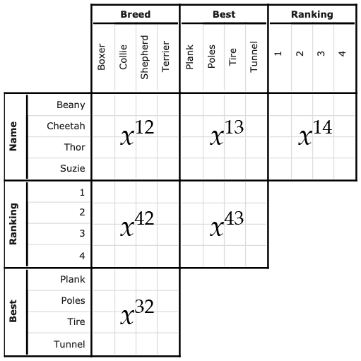
Figure 2: Figure from https://www.brainzilla.com, modified to show grid mapping
First, we will add the extra grids and place the row-column constraints on them as we did before. Because of the way we have chosen to write our model, extending it to 4 variables (which yields 3 additional grids) means we can build on what we already have:
model4 <- model3 |>
  # 3 additional grids:
  add_variable(x14[i, j], i = 1:n, j = 1:n, type = "binary") |>
  add_variable(x42[i, j], i = 1:n, j = 1:n, type = "binary") |>
  add_variable(x43[i, j], i = 1:n, j = 1:n, type = "binary") |>

  # Only one cell can be assigned in a row, as before:
  add_constraint(sum_expr(x14[i, j], j = 1:n) == 1, i = 1:n) |>
  add_constraint(sum_expr(x42[i, j], j = 1:n) == 1, i = 1:n) |>
  add_constraint(sum_expr(x43[i, j], j = 1:n) == 1, i = 1:n) |>

  # Only one cell can be assigned in a column, as before:
  add_constraint(sum_expr(x14[i, j], i = 1:n) == 1, j = 1:n) |>
  add_constraint(sum_expr(x42[i, j], i = 1:n) == 1, j = 1:n) |>
  add_constraint(sum_expr(x43[i, j], i = 1:n) == 1, j = 1:n) |>

  # Additional logic:
  add_constraint(x12[i, j] + x14[i, k] <= x42[k, j] + 1, i = 1:n, j = 1:n, k = 1:n) |>
  add_constraint(x13[i, j] + x14[i, k] <= x43[k, j] + 1, i = 1:n, j = 1:n, k = 1:n) |>
  add_constraint(x42[i, j] + x43[i, k] <= x32[k, j] + 1, i = 1:n, j = 1:n, k = 1:n)
With the model specified, we can now translate the clues into constraints. You might recall that one of the clues is “The Boxer (1) ranked 1 position after the Shepherd (3)”, which we can’t specify in a fixed way. The key here will be to utilize the
model4_fixed <- model4 |>
  # 2. The Boxer (1) ranked 1 position after the Shepherd (3):
  add_constraint(x42[1, 1] == 0) |> # Boxer cannot be 1st
  add_constraint(x42[4, 3] == 0) |> # Shepherd cannot be 4th
  add_constraint(sum_expr(i * x42[i, 1], i = 1:4) == sum_expr(i * x42[i, 3], i = 1:4) + 1) |>
  #    None of them likes the tunnel (4), nor jumping through the tire (3):
  add_constraint(x32[i, 1] == 0, i = 3:4) |> # Boxer's dislikes
  add_constraint(x32[i, 3] == 0, i = 3:4) |> # Shepherd dislikes

  # 3. Cheetah (2) and the dog who loves the poles (2) were 1st and 3rd:
  add_constraint(x13[2, 2] == 0) |> # Cheetah cannot like poles
  add_constraint(x14[2, 1] == 1) |> # Cheetah is in 1st position
  add_constraint(x43[3, 2] == 1) |> # Dog who loves poles is in 3rd

  # 1. Only the winning dog has the same initial letter in name and breed:
  add_constraint(x12[2, 2] == 1) |> # Therefore Cheetah is a Collie
  add_constraint(x12[1, 1] == 0) |> # and Beany cannot be a Boxer
  add_constraint(x12[3, 4] == 0) |> # and Thor cannot be a Terrier
  add_constraint(x12[4, 3] == 0) |> # and Suzie cannot be a Shepherd

  # 4. Thor (3) doesn't like the plank (1) and didn't come 2nd:
  add_constraint(x13[3, 1] == 0) |>
  add_constraint(x14[3, 2] == 0) |>

  # 5. Cheetah (2) either loves the tunnel (4) or she came 4th:
  add_constraint(x13[2, 4] == 1) |> # Since Cheetah came 1st, she must love the tunnel

  # 6. The dog who loves the plank (1) came 1 position after the dog who loves the poles (2):
  add_constraint(x42[1, 1] == 0) |> # Plank cannot be 1st
  add_constraint(x42[4, 2] == 0) |> # Poles cannot be 4th
  add_constraint(sum_expr(i * x43[i, 1], i = 1:4) == sum_expr(i * x43[i, 2], i = 1:4) + 1) |>

  # 7. Suzie (4) is not a Shepherd (3) and Beany (1) doesn't like the tunnel (4):
  add_constraint(x12[4, 3] == 0)
  # We don't need anymore constraints because tunnel is already claimed by Cheetah
result4 <- solve_model(model4_fixed, with_ROI(solver = "glpk", verbose = TRUE))
## <SOLVER MSG>  ----
## GLPK Simplex Optimizer 5.0
## 325 rows, 96 columns, 995 non-zeros
##       0: obj =  -0.000000000e+00 inf =   5.400e+01 (54)
##      78: obj =  -0.000000000e+00 inf =   9.437e-15 (0)
## OPTIMAL LP SOLUTION FOUND
## GLPK Integer Optimizer 5.0
## 325 rows, 96 columns, 995 non-zeros
## 96 integer variables, all of which are binary
## Integer optimization begins...
## Long-step dual simplex will be used
## +    78: mip =     not found yet <=              +inf        (1; 0)
## +    83: >>>>>   0.000000000e+00 <=   0.000000000e+00   0.0% (1; 1)
## +    83: mip =   0.000000000e+00 <=     tree is empty   0.0% (0; 3)
## INTEGER OPTIMAL SOLUTION FOUND
## <!SOLVER MSG> ----
Is <- c("Beany", "Cheetah", "Thor", "Suzie") # name
Js <- c("Boxer", "Collie", "Shepherd", "Terrier") # breed
Ks <- c("Plank", "Poles", "Tire", "Tunnel") # best at
Ls <- as.character(1:4) # ranking

# Extract solved grids:
solution4 <- list(
  x12 = get_solution(result4, x12[i, j]) |>
    filter(value == 1) |>
    select(-c(variable, value)) |>
    mutate(i = Is[i], j = Js[j]),
  x13 = get_solution(result4, x13[i, k]) |>
    filter(value == 1) |>
    select(-c(variable, value)) |>
    mutate(i = Is[i], k = Ks[k]),
  x14 = get_solution(result4, x14[i, l]) |>
    filter(value == 1) |>
    select(-c(variable, value)) |>
    mutate(i = Is[i], l = Ls[l]),
  x42 = get_solution(result4, x42[l, j]) |>
    filter(value == 1) |>
    select(-c(variable, value)) |>
    mutate(l = Ls[l], j = Js[j]),
  x43 = get_solution(result4, x43[l, k]) |>
    filter(value == 1) |>
    select(-c(variable, value)) |>
    mutate(l = Ls[l], k = Ks[k]),
  x32 = get_solution(result4, x32[k, j]) |>
    filter(value == 1) |>
    select(-c(variable, value)) |>
    mutate(k = Ks[k], j = Js[j])
)
This is the solution we would obtain by elimination:
| Dog | Breed | Best | Position |
|---|---|---|---|
| Beany | Terrier | Tire | 2 |
| Cheetah | Collie | Tunnel | 1 |
| Suzie | Boxer | Plank | 4 |
| Thor | Shepherd | Poles | 3 |
This is the solution found by the computer:
solution4 |>
  reduce(left_join) |>
  arrange(i) |>
  kable(col.names = c("Dog", "Breed", "Best", "Position"), align = "l")
| Dog | Breed | Best | Position |
|---|---|---|---|
| Beany | Terrier | Tire | 2 |
| Cheetah | Collie | Tunnel | 1 |
| Suzie | Boxer | Plank | 4 |
| Thor | Shepherd | Poles | 3 |
Further reading and other software
OMPR was inspired by JuMP modeling language and collection of packages for mathematical optimization in Julia. If you are interested in mathematical modeling and optimization in Python, check out Pyomo. (And its documentation.)
This post from Jeff Schecter is an insightful introduction to constrained optimization (using Pyomo) with the application of matching clients with stylists at Stitch Fix.
-
See this article ↩︎
-
For that I would recommend these articles in its documentation. ↩︎
-
add_constraint(model3, x12[i, j] * x13[i, k] == x32[k, j], i = 1:n, j = 1:n, k = 1:n), while intuitive, results in the following error:Error in x12[i, j] * x13[i, k] : non-numeric argument to binary operator↩︎
- Posted on:
- May 4, 2019
- Length:
- 13 minute read, 2588 words