Bayesian Optimization in R

Update (2022-05-01): I redid all of the graphics with ggplot2 and all of the animated GIFs with gganimate.

Introduction

Optimization of function $f$ is finding an input value ${\mathbf{x}}_{\ast }$ which minimizes (or maximizes) the output value:

$$\begin{array}{r}{\mathbf{x}}_{\ast }=\underset{\mathbf{x}}{\arg min}f(\mathbf{x})\end{array}$$

In this tutorial we will optimize a function from Forrester et. al (2008):

$$f(x)=(6x-2{)}^2\text{sin}(12x-4),$$

which looks like this when $x\in [0,1]$:

ggplot() +
  geom_function(
    fun = \(x) (6 * x - 2)^2 * sin(12 * x - 4)
  ) +
  xlim(0, 1)

The ideal scenario is that $f$ is known, has a closed, analytical form, and is differentiable – which would enable us to use gradient descent-based algorithms. For example, here’s how we might optimize it with Adam in torch:

library(torch)

x <- torch_zeros(1, requires_grad = TRUE)
f <- function(x) (6 * x - 2) ^ 2 * torch_sin(12 * x - 4)

optimizer <- optim_adam(x, lr = 0.25)

for (i in 1:50) {
  y <- f(x)
  optimizer$zero_grad()
  y$backward()
  optimizer$step()
}

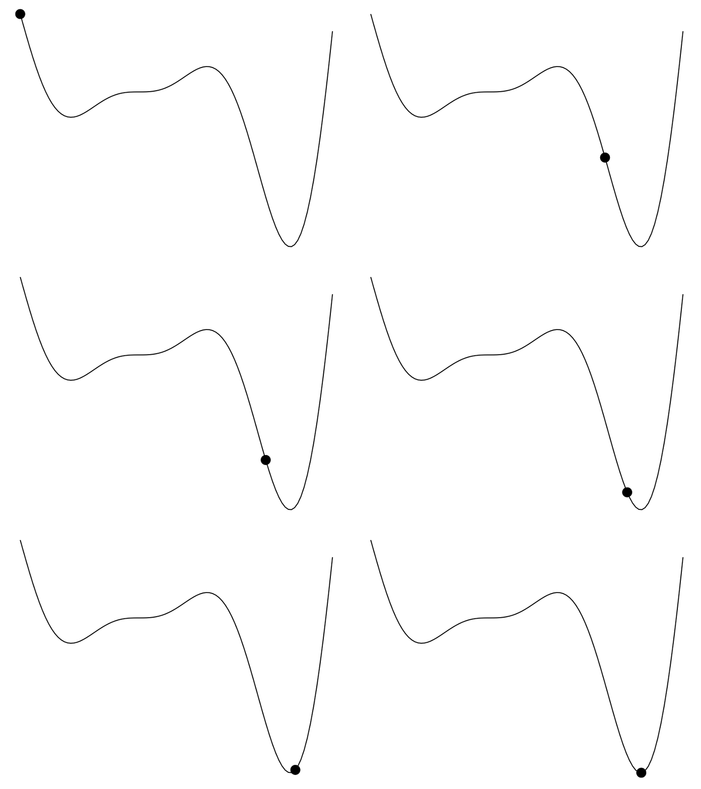
But that’s not always the case. Maybe we don’t have a derivative to work with and the evaluation of the function is expensive – hours to train a model or weeks to do an A/B test. Bayesian optimization (BayesOpt) is one algorithm that helps us perform derivative-free optimization of black-box functions.

Algorithm

The BayesOpt algorithm for $N$ maximum evaluations can be described using the following pseudocode:

Place Gaussian process prior on 'f'
Observe 'f' at n0 initial points; set n = n0
while n ≤ N do:
  Update posterior on 'f' using all available data
  Compute acqusition function 'a' using posterior
  Let x* be the value which maximizes 'a'
  Observe f(x*)
  Increment n
end while
Return x for which f(x) was at its best

We seed the algorithm with a few initial evaluations and then proceed to sequentially find and evaluate new values, chosen based on some acquisition function, until we’ve exhausted the number of attempts we’re allowed to make.

Acquisition functions

Let $y_{\text{best}}$ be the best observed value of $f_n$ (the $n$ evaluations of $f$). How do we choose the next value at which to evaluate $f$? We use an acquisition function to guide our choice. There are three major acquisition functions out there, each with its own pros and cons:

1. Probability of improvement (least popular): $a_{\text{PI}}(x)$ measures the probability that a point $x$ will lead to an improvement over $y_{\text{best}}$
2. Expected improvement (most popular): $a_{\text{EI}}$ incorporates the amount of improvement over $y_{\text{best}}$
3. GP lower confidence bound (newer of the three): $a_{\text{LCB}}$ (upper in case of maximization) balances exploitation (points with best expected value) against exploration (points with high uncertainty).

In the sections below, each acquisition function will be formally introduced and we’ll see how to implement it in R.

Implementation

We will use the GPfit package for working with Gaussian processes.

library(GPfit) # install.packages("GPfit")
library(dplyr)

## Warning: package 'dplyr' was built under R version 4.2.3

library(tidyr)

## Warning: package 'tidyr' was built under R version 4.2.3

library(purrr)

The algorithm is executed in a loop:

for (iteration in 1:max_iterations) {
  # step 1: fit GP model to evaluated points
  # step 2: calculate utility to find next point
}

f <- function(x) {
  return((6 * x - 2)^2 * sin(12 * x - 4))
}

We start with $n_0$ equally-spaced points between 0 and 1 on which to evaluate $f$ (without noise) and store these in a matrix evaluations:

# seed with a few evaluations:
n0 <- 4
evaluations <- matrix(
  as.numeric(NA),
  ncol = 2, nrow = n0,
  dimnames = list(NULL, c("x", "y"))
)
evaluations[, "x"] <- seq(0, 1, length.out = n0)
evaluations[, "y"] <- f(evaluations[, "x"])

evaluations

GP model fitting

In this example we are going to employ the popular choice of the power exponential correlation function, but the Màtern correlation function list(type = "matern", nu = 5/2) may also be used.

set.seed(20190416)

fit <- GP_fit(
  X = evaluations[, "x"],
  Y = evaluations[, "y"],
  corr = list(type = "exponential", power = 1.95)
)

Now that we have a fitted GP model, we can calculate the expected value $\mu (x)$ at each possible value of $x$ and the corresponding uncertainty $\sigma (x)$. These will be used when computing the acquisition functions over the possible values of $x$.

yhat <- predict.GP(
    fit,
    xnew = data.frame(x = seq(0, 1, length.out = 100))
  )$complete_data |>
  as.data.frame() |>
  rename(x_new = xnew.1, mu = Y_hat) |>
  mutate(sigma = sqrt(MSE))

yhat_plot <- yhat |>
  ggplot() +
  geom_ribbon(aes(x = x_new, ymin = mu - sigma, ymax = mu + sigma), alpha = 0.2) +
  geom_line(aes(x = x_new, y = mu), linetype = "dashed") +
  geom_point(
    data = as.data.frame(evaluations),
    aes(x = x, y = y),
    size = 2
  ) +
  ggtitle("GP model fit with 4 data points")

yhat_plot

Calculating utility

As mentioned before, suppose $y_{\text{best}}$ is the best evaluation we have so far:

y_best <- min(evaluations[, "y"])

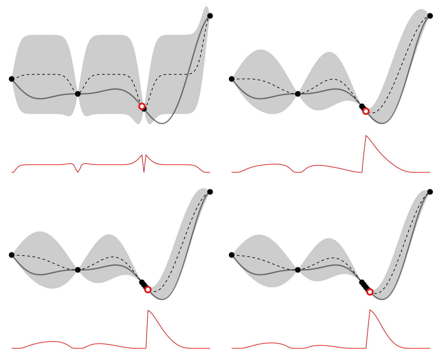
Probability of improvement

This utility measures the probability of improving upon $y_{\text{best}}$, and – since the posterior is Gaussian – we can compute it analytically:

$$a_{\text{POI}}(x)=\mathrm{\Phi }\left(\frac{y_{\text{best}}-\mu (x)}{\sigma (x)}\right)$$

where $\mathrm{\Phi }$ is the standard normal cumulative distribution function. In R, it looks like this:

probability_improvement <- tibble(
  x = yhat$x_new,
  prob_improve = map2_dbl(
    yhat$mu,
    yhat$sigma,
    function(m, s) {
      if (s == 0) return(0)
      else {
        poi <- pnorm((y_best - m) / s)
        # poi <- 1 - poi (if maximizing)
        return(poi)
      }
    }
  )
)

probability_improvement_plot <- probability_improvement |>
  ggplot() +
  geom_line(aes(x = x, y = prob_improve), color = "#E41A1C") +
  ggtitle("Probability of improvement")

yhat_plot +
  probability_improvement_plot +
  plot_layout(ncol = 1)

Using this acquisition function, the next point which should be evaluated is:

probability_improvement |>
  top_n(1, prob_improve) |>
  pull(x)

## [1] 0.6565657

Expected improvement

Let $\gamma (x)$ be the quantity we used in $a_{\text{POI}}$:

$$\gamma (x)=\frac{y_{\text{best}}-\mu (x)}{\sigma (x)}$$

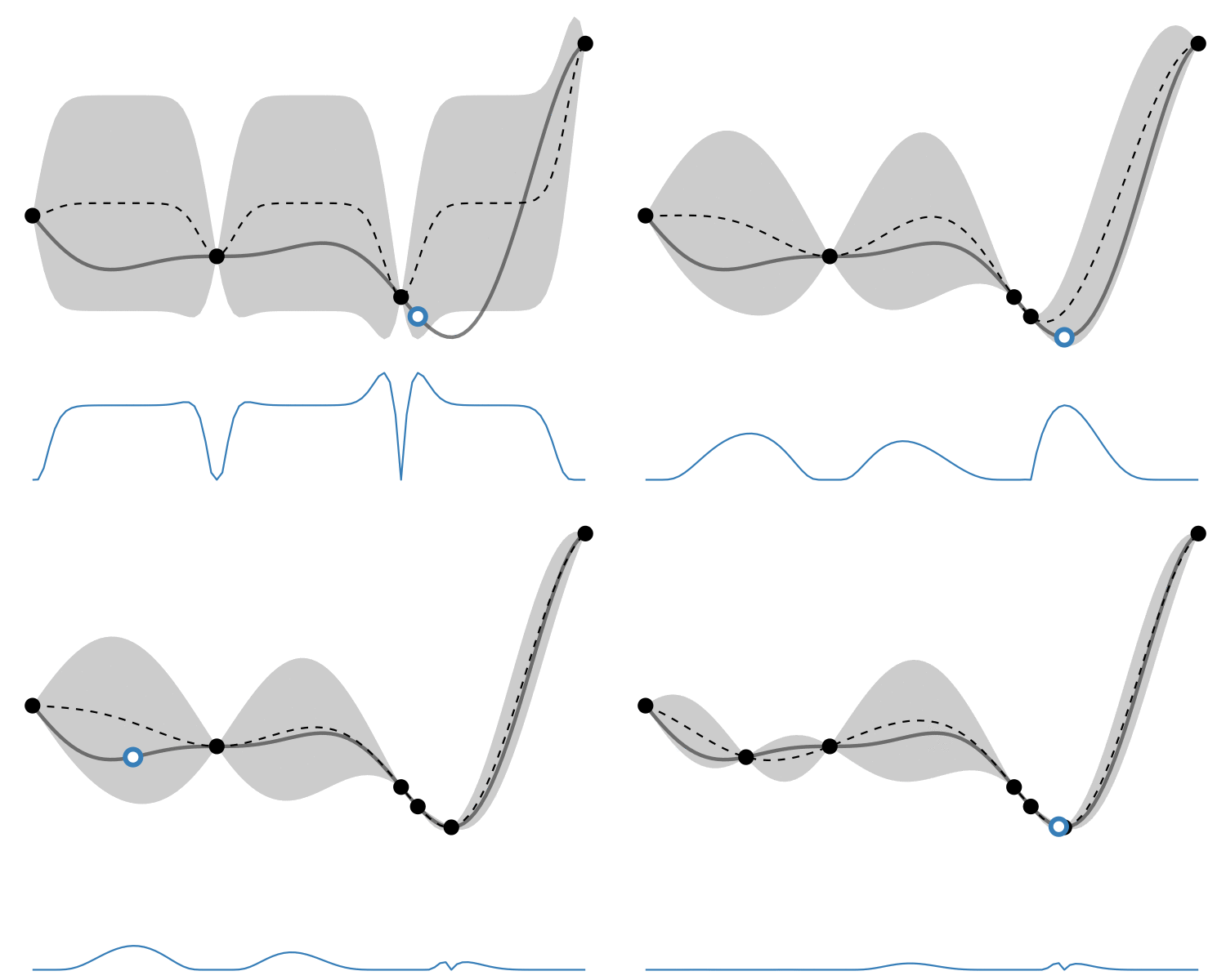
Building on probability of improvement, this utility incorporates the amount of improvement:

$$a_{\text{EI}}=\sigma (x)(\gamma (x)\mathrm{\Phi }(\gamma (x))+\mathcal{N}(\gamma (x);0,1))$$

In R, it looks like this:

expected_improvement <- tibble(
  x = yhat$x_new,
  expect_improve = map2_dbl(
    yhat$mu,
    yhat$sigma,
    function(m, s) {
      if (s == 0) return(0)
      gamma <- (y_best - m) / s
      phi <- pnorm(gamma)
      return(s * (gamma * phi + dnorm(gamma)))
    }
  )
)

expected_improvement_plot <- expected_improvement |>
  ggplot() +
  geom_line(aes(x = x, y = expect_improve), color = "#377EB8") +
  ggtitle("Expected improvement")

yhat_plot +
  expected_improvement_plot +
  plot_layout(ncol = 1)

Using this acquisition function, the next point which should be evaluated is:

expected_improvement |>
  top_n(1, expect_improve) |>
  pull(x)

## [1] 0.6969697

GP lower confidence bound

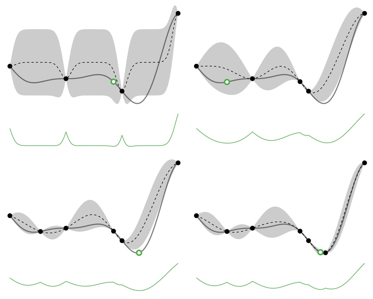
As mentioned above, this utility enables us to control whether the algorithm prefers exploitation – picking points which have the best expected values – or exploration – picking points which have the highest uncertainty, and this would be more informative to evaluate on. This balance is controlled by a tunable hyperparameter $\kappa$, and in R it looks like:

kappa <- 2 # tunable
lower_confidence_bound <- tibble(
  x = yhat$x_new,
  lcb = yhat$mu - kappa * yhat$sigma
)

lower_confidence_bound_plot <- lower_confidence_bound |>
  ggplot() +
  geom_line(aes(x = x, y = lcb), color = "#4DAF4A") +
  ggtitle("Lower confidence bound")

yhat_plot +
  lower_confidence_bound_plot +
  plot_layout(ncol = 1)

Using this acquisition function, the next point which should be evaluated is:

lower_confidence_bound |>
  top_n(1, desc(lcb)) |>
  pull(x)

## [1] 0.6161616

Comparison

So how different are the results? Let’s how the choice of acquisition function affects the journey the BayesOpt algorithm takes over the course of 5 iterations:

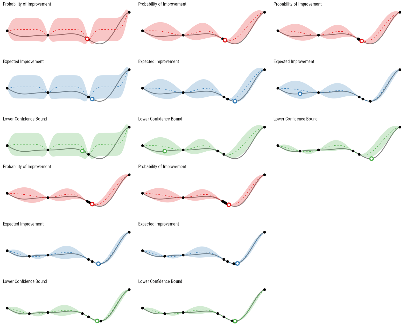
In this example we arrive at more-or-less the same destination no matter which path we take.

Closing thoughts

This was only a one-dimensional optimization example to show the key ideas and how one might implement them. If you are interested in using this algorithm to tune your models’ parameters, I encourage you to check out this documentation which describes how to perform Bayesian optimization with Pyro (the probabilistic programming language built on PyTorch); and pyGPGO, which is a Bayesian optimization library for Python.

Update 2019-09-30: Not long after I published this tutorial, Meta AI open-sourced GPyTorch-based BoTorch and “adaptive experimentation platform” Ax. Refer to ai.facebook.com for more details.

Further reading

• Practical Bayesian Optimization of Machine Learning Algorithms
• Taking the Human Out of the Loop: A Review of Bayesian Optimization
• Bayesian Optimization in AlphaGo
• Gaussian processes
  • A Visual Exploration of Gaussian Processes
  • Gaussian Process, not quite for dummies
  • Implementing Gaussian Process in Python and R
  • Un garçon pas comme les autres (Bayes): Yes but what is a Gaussian process? or, Once, twice, three times a definition; or A descent into madness
• Constrained Bayesian Optimization with Noisy Experiments

References

Forrester, Sobester, A. 2008. Engineering Design via Surrogate Modelling: A Practical Guide. Wiley.
Frazier, Peter I. 2018. “A Tutorial on Bayesian Optimization.” arXiv.org, July. https://arxiv.org/abs/1807.02811.
Kingma, Diederik P, and Jimmy Ba. 2014. “Adam: A Method for Stochastic Optimization.” arXiv.org, December. https://arxiv.org/abs/1412.6980.
- Posted on:
- April 16, 2019
- Length:
- 8 minute read, 1568 words